Identifying that an object exists somewhere in an image is one thing. Tracing its exact outline, pixel by pixel, separating it precisely from everything around it, is something else entirely. The history of image segmentation is the story of that second, much harder problem, and it spans from simple mathematical thresholds applied to grayscale images to deep learning systems capable of producing pixel-perfect masks for every object, and every category of background, in a complex scene. This article traces that history from its earliest techniques to the panoptic segmentation frameworks used today.
What Image Segmentation Actually Means
Pixel-level classification mask is the core concept underlying the history of image segmentation. Rather than describing an image with a single label, or even with bounding boxes around objects as in the history of object detection, segmentation produces an output where every single pixel in an image is assigned to a category, an object, a type of surface, the sky, or any other relevant class.
This task connects directly to the broader history of computer vision, since segmentation has always required understanding not just what is present in an image, but precisely where the boundaries between different elements lie, a problem closely related to but distinct from the history of edge detection.
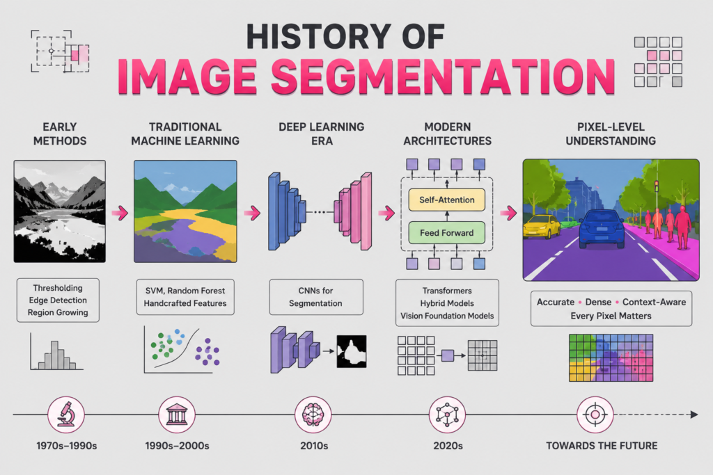
Early Approaches: Thresholding and Region Growing (1970 – 1990)
Traditional image thresholding history represents one of the earliest and simplest approaches to image segmentation. Thresholding works by selecting a brightness value and classifying every pixel as belonging to one of two categories, depending on whether its intensity falls above or below that threshold. Background vs foreground separation, one of the most fundamental segmentation tasks, could often be achieved using thresholding in images with simple, high-contrast content, such as a dark object against a bright background.
This approach connects to the broader first computer vision experiments of the 1960s and the techniques developed throughout the history of image processing during the 1970s, where simple mathematical operations applied to pixel values could produce surprisingly useful results for constrained problems.
Watershed segmentation algorithm historical background represents a more sophisticated approach developed during this period. The watershed algorithm treats an image as a topographic surface, where pixel intensity values correspond to elevation, and simulates a flooding process, identifying regions, watersheds, that would collect water from different points, effectively segmenting the image into regions separated by ridge lines corresponding to significant intensity changes.
Active Contours and Energy Minimization (1987 – 2000)
History of active contour models snake algorithm marks a significant conceptual development. Introduced in the late 1980s, active contour models, often called snakes, work by initializing a curve somewhere within an image and then iteratively deforming that curve to minimize an energy function. This energy function typically balances two competing goals: the curve should be smooth, and the curve should align with strong edges or boundaries within the image, connecting this approach directly to the history of edge detection.
This iterative, optimization-based approach to segmentation represented a meaningful step beyond simple thresholding, since it could adapt to more complex and irregular boundaries than a fixed intensity threshold could capture. However, active contour models generally required reasonable initialization, a starting curve placed somewhere near the actual boundary of interest, and could struggle with images containing significant noise or multiple overlapping objects.
Graph-Based and Statistical Approaches (1990 – 2010)
From graph cuts to deep image segmentation describes an important transitional period in the history of image segmentation. Graph cut approaches represented images as graphs, where pixels were treated as nodes and connections between neighboring pixels were weighted based on their similarity. Segmentation then became a problem of finding the optimal way to cut this graph into separate regions, minimizing some measure of dissimilarity within regions while maximizing dissimilarity between regions.
Evolution of mean shift segmentation software during this period represented a different statistical approach, treating segmentation as a problem of finding clusters in a feature space representing pixel colors and positions. Mean shift identified modes, or peaks, in this feature space and assigned pixels to the cluster corresponding to the nearest mode, producing segments based on color and spatial proximity without requiring a predetermined number of segments.
Superpixel generation mechanics emerged as a related but distinct concept during this period. Rather than attempting to segment an entire image into final, meaningful regions directly, superpixel algorithms grouped pixels into small, perceptually meaningful clusters, superpixels, that respected local image boundaries. These superpixels could then serve as a more efficient and meaningful unit for subsequent processing than individual pixels, reducing computational complexity for later stages of analysis.
This period overlapped significantly with the broader history of pattern recognition, as segmentation increasingly incorporated statistical and machine learning techniques rather than relying purely on hand-designed geometric or intensity-based rules.
Deep Learning Transforms Segmentation (2014 – 2017)
History of semantic segmentation neural networks begins in earnest following the broader deep learning transformed computer vision revolution that started with the history of AlexNet in 2012. Fully Convolutional Networks (FCN), introduced around 2014 and 2015, represented a foundational architecture for this transition.
FCNs adapted convolutional neural network architectures, originally designed for classification, by replacing the final fully connected layers with convolutional layers that produced an output the same spatial size as the input image, with each pixel in this output representing a classification for the corresponding pixel in the input. This was a significant conceptual shift: rather than producing a single classification for an entire image, the network produced a dense, pixel-level classification map, directly addressing the pixel-level classification mask goal of segmentation.
SegNet and DeepLab models built on this foundation with architectural refinements. SegNet introduced an encoder-decoder structure, where the encoder progressively reduced the spatial resolution of the input while extracting increasingly abstract features, and the decoder progressively restored the spatial resolution, producing a final segmentation map at the same resolution as the input image.
Spatial pyramid pooling (ASPP), Atrous Spatial Pyramid Pooling, became an important technique within models like DeepLab, allowing the network to capture information at multiple scales simultaneously by applying convolutions with different dilation rates, effectively examining the image at multiple effective resolutions without requiring multiple separate processing pathways.
Instance Segmentation: Telling Objects Apart (2017 – 2020)
Development of instance segmentation techniques addresses an important limitation of semantic segmentation as described so far. Semantic segmentation classifies every pixel according to its category, but does not distinguish between multiple separate instances of the same category, two cars in an image might both be classified as “car” without any indication that they are two distinct objects.
Mask R-CNN development, building directly on the history of faster r-cnn, addressed this limitation by combining object detection with segmentation. For each detected object, Mask R-CNN produced not just a bounding box and class label, but also a pixel-level mask specific to that individual object instance, allowing the system to distinguish between multiple objects of the same category within an image, each with its own precise segmentation mask.
This connects directly to the broader history of object detection, demonstrating how architectural advances in detection, particularly the region-based approaches descended from the history of r-cnn, could be extended to address segmentation tasks as well, illustrating the close relationship between these two areas of computer vision research.
Medical Imaging and U-Net (2015 – 2026)
History of U-Net medical image segmentation represents one of the most influential and widely cited architectures within the broader history of image segmentation. Introduced in 2015 specifically for biomedical image segmentation tasks, U-Net used an encoder-decoder structure with skip connections, direct connections between corresponding layers in the encoder and decoder, that helped preserve fine spatial details that might otherwise be lost during the encoding process.
U-Net proved particularly effective for medical imaging ai applications, where precise segmentation of structures like organs, tumors, or cellular components can be critical for diagnosis and treatment planning. The architecture’s effectiveness, combined with its relative simplicity compared to some alternatives, made it one of the most widely adapted segmentation architectures, with countless variants developed for specific medical and non-medical applications alike.
Dice coefficient validation and Jaccard index similarity became standard metrics for evaluating segmentation quality during this period, both measuring the overlap between a predicted segmentation mask and a ground truth mask, providing quantitative ways to compare different segmentation approaches and track improvements over time.
Panoptic Segmentation: Unifying the Approaches (2018 – 2026)
History of panoptic segmentation frameworks represents a more recent unification within the history of image segmentation. Panoptic segmentation combines semantic segmentation, classifying every pixel by category, including background categories like sky or road that don’t correspond to distinct countable objects, with instance segmentation, distinguishing between individual instances of countable object categories like cars or people.
This unified approach reflects a broader trend toward comprehensive scene understanding, connecting to applications including self-driving cars and computer vision, where understanding both the overall layout of a scene, road, sidewalk, sky, and the individual objects within it, vehicles, pedestrians, cyclists, each as distinct instances, is essential for safe navigation.
Boundary refinement processing has continued to develop alongside these architectural advances, addressing the persistent challenge of producing segmentation masks with precise, accurate boundaries, particularly for objects with fine details or complex shapes, an area where vision transformers have also shown promising results, bringing global context to bear on the boundary refinement problem in ways that purely convolutional approaches sometimes struggled with.
Frequently Asked Questions
What is the difference between image segmentation and object detection?
Object detection identifies objects within an image and draws bounding boxes around them, providing a rectangular approximation of an object’s location. Image segmentation goes further, classifying every individual pixel in an image, producing precise outlines of objects and other regions rather than rectangular approximations.
What is the difference between semantic and instance segmentation?
Semantic segmentation classifies every pixel according to its category, such as road, sky, or car, without distinguishing between multiple objects of the same category. Instance segmentation goes further, distinguishing between individual instances of the same category, so that two cars in an image are identified as two separate objects, each with its own segmentation mask.
What is U-Net and why is it important for medical imaging?
U-Net is a segmentation architecture introduced in 2015, using an encoder-decoder structure with skip connections that help preserve fine spatial detail. It has proven particularly effective for medical image segmentation tasks, where precisely outlining structures like organs or tumors is critical, and remains one of the most widely adapted segmentation architectures.
What is panoptic segmentation?
Panoptic segmentation combines semantic segmentation, which classifies every pixel by category including background regions, with instance segmentation, which distinguishes between individual instances of countable objects. This provides a unified, comprehensive understanding of a scene, useful for applications like autonomous driving where both overall scene layout and individual object identification matter.
How is segmentation quality measured?
Segmentation quality is commonly measured using metrics like the Dice coefficient and the Jaccard index, both of which quantify the overlap between a predicted segmentation mask and a ground truth mask. Higher values indicate greater overlap and therefore more accurate segmentation.
Conclusion
The history of image segmentation traces a path from simple intensity thresholds and region-growing algorithms, through energy-minimizing active contours and graph-based statistical methods, to deep learning architectures capable of producing precise, pixel-level classifications for entire scenes. Each step addressed limitations of what came before, eventually arriving at unified frameworks like panoptic segmentation that combine multiple types of scene understanding into a single output.
Within the broader story of computer vision technology, image segmentation represents one of the clearest examples of a problem that seems conceptually simple, label every pixel, but that required decades of mathematical, algorithmic, and architectural innovation to solve effectively across the enormous diversity of real-world images. Understanding the history of image segmentation means understanding how AI learned not just to see what is in an image, but to trace its exact shape, pixel by pixel.